Dynamics IV – 1 In Perspective

Download this tutorial in PDF format (0.4 Mb).

As a decent mutual understanding is key in maintaining good relationships, I wrote Poser Features in Perspective to give you some historic background on various Poser functions that receive a lot of debate. Cloth Room, FireFly rendering and the evolution of the Vicky and Mike characters, for instance. Especially Poser users discussing the future might be interested in some history.

For those curious about the peculiarities of cloth simulation in general, I added Cloth Simulation in Perspective. It’s mainly about the behavior of 3D meshes for cloth, so especially Dynamic Garment Makers (virtual tailors) might be interested.

Dynamics IV – 2 Poser features in perspective

The history of Poser is rather well documented in Wikipedia. Just a brief overview:

1	1995	Fractal design
2	1996	Fractal design	Props, Animation
3	1998	MetaCreations	User Interface (the Bryce-like), Expressions, Hand poses
4	1999	MetaCreations	Sketch render, Transparency, Conforming clothes, Magnets
ProPack	2000	Curious Labs	Python scripting, custom rigging (now: setup room)
5	2003	Curious Labs	Firefly render, Collision detection, Dynamic hair & cloth
6	2005	e-Frontier	OpenGL, IBL, Cartoon render
7	2006	e-Frontier	Talk designer, multithreading, HDRI, Morphing brush, universal poses

MetaCreations was a merger of the people from Poser, from Bryce, from Painter, from RayDream/InfiniD, from Kai’s Power Tools and alike. Thanks to this, Bryce was able to handle Poser files from the early days on, and thanks to Kai Krause, they both have a similar user interface. When MetaCreations broke up, Bryce and Painter went to Corel who later sold Bryce to DAZ. InfiniD went to Eovia to become Carrara, which later ended up at DAZ as well. The Poser people continued as Curious Labs.

Establishing Poser 5 however turned into a shear disaster (well described by John (Vanishing Point) Hoagland himself in http://www.cocs.com/poser/poser5mess.htm) and e-Frontier took over. After a while they sold their entire American branch to Smith Micro (founded by William Smith Jr). The Japanese branch is still known for the 3D modeler “Shade” and still represents the Japanese version of Poser. From then on Poser is in the hands of Smith Micro, Poser Pro gets introduced, and functionality has increased a lot since.

For a better understanding of the advanced features like Cloth Room and FireFly, it pays off to elaborate a bit on that hectic period around the turn of the century. Let’s take a look from the other side.

Reyes

In January 1996 the writer/producer Jorge Martinez Reverte, Javier Reyes and Jose Maria De Espona formed a company REM Infografica, based in Madrid, Spain. REM was the acronym of Reyes Espona Martinez. Martinez became CEO, Reyes became Technical/R&D Director and De Espona became the Art & Production director for the 3D Models Databank. (source: www.deespona.com/personalweb).

A sequence of splits and mergers (1998) moved the modelbank to Viewpoint (later: Digimation), created Next Limit (RealFlow) and also Reyes Infografica, known from 3DS Max plugins like Cloth:Reyes, Cartoon:Reyes, NPR:Reyes and more. In 2000 the latter sold its plugin technology for use in Poser. Cartoon:Reyes became Poser Toon render (the Sketch render was already available in Poser 4), NPR:Reyes became the Poser FireFly render, Cloth:Reyes became Cloth Room and so on. Javier Reyes himself continued with Virtual Fashion, until that came to its own end as a product (say 2009).

Some background references:

http://www.cgarena.com/archives/interviews/3daliens/interview.html on the foundation of Next Limit
http://forums.cgsociety.org/archive/index.php/t-725233.html Reyes Infografica doing plugins for Max 2 (1998, I was into 3DS Max myself, those days).
3DS Max moves to Kinetix (Max 3, 1999) which then moves to Discreet (Max 4, 2000). From 2001 on, the Reyes plugins were not supported anymore
http://forums.cgsociety.org/archive/index.php/t-725233.html
http://forums.cgsociety.org/archive/index.php/t-1006.html
3DS MAX 5 introduced a completely renewed set of… rendering features.

So now we know where those Poser modules came from, and why creating Poser 5 took so much trouble: a lot of (Spanish?) 3DS max plugins had to be integrated in the Poser 4 framework. In the meanwhile, sometimes some confusion passes by.

The rendering module
The NPR:Reyes (NPR = Non Photoreal Render) aka FireFly render is based on the initial Renderman REYES technology, where REYES is an acronym for Render Everything Your Eyes (can) See. The Reyes from Infografica is just a normal Spanish name. In the NPR:Reyes product, the two came together.
REYES was a serious improvement over the scanline rendering (Poser 4, 3DS Max) without the enormous calculation times from the raytracers in those days, and with the ability to chop rendering tasks in pieces to support large scale projects. It did not support extensive raytracing (*) but offered speedy alternatives (environment mapping) instead. Later on, Pixar enhanced the Renderman techniques by adding explicit raytracing to create their own PhotoRealistic Renderman toolkit.
So it might come as a shock to you, but FireFly is not raytracing very well. By design.

(*) for the tech’s amongst you: classical raytracing techniques scatter rays of light throughout the scene, and must consider the scene, and the objects, as a whole to do so. The REYES algorithm on the other hand chops a scene into chunks (buckets) and then into very tiny pieces (micropolygons) in an early stage. So both treat the scene geometry in opposite ways. As a result, REYES based renderers have problems with raytracing, and raytracing renderers have problems with performance.

A view on characters

So, the introduction of Poser 5 was a milestone in its history, and a heavy one. Next to the software and its functions, it had impact on content and future developments as well. Up till then, DAZ had created the Vicky and Mike characters (versions 1 and 2) based on the P4 female and male, which as such were Zygothe products. The turnover to Poser 5 brought some serious licensing issues between MetaCreations and DAZ, and the latter decided to go their own way.

This own way introduced the unimesh geometry, the wish to create all characters from one single mesh. Vicky and Mike 3 introduced that concept, soon to be followed by Stephanie 3 which was a real-person body scan translated to the unimesh. DAZ also had their own view on the software, which brought us Daz Studio consisting of a free base with paid plugins – just a completely different marketing concept compared to Poser.
Boths DAZ views developed, and after a successful rebuild of Vick and Mike 4 using the new modo modeler, and after successfully turning Girl 4, Steph 4 and so on into morphs of Vickys mesh, DAZ launched Genesis – the new generation unimesh, with all known figures (Vick and Mike 5 included) provided as morphs of that base mesh, and including a serious Poser contender Daz Studio 4, at the turn of 2011/2012. The weight-mapping mechanisms for smoother posing forced Smith Micro into similar features for Poser 9 / Pro 2012. But mainly, the full features of the new DAZ characters could not be deployed in Poser at the fullest, you needed DS4 for that.
This came as a serious chock to the Poser community. Being “Poser-compatible” was not the default anymore.

There is always more (on clothing)

Around the turn of the century, Serge Marck published his site www.poserfashion.net (before it got hacked, you can find the Original in Internet’s WayBackMachine). He published clothes for Poser 4 (conforming), Poser 5 (some dynamic for V3) and Poser 6 (dynamic, V4).He was into cloth simulation for some time already, and discussed SimCloth, Cloth:Reyes, ClothFX and Maya/Cloth. Apparently the relevant products in those days.

SimCloth is still around as a Max plugin. It’s opensource, so just go http://www.spot3d.com/simcloth/ and get the code, if you like. That is, if you want to find out about the internals. It’s created by Vladimir Koylazov (Vlado) in 2000 – 2002, and got a serious update in 2005. Vlado himself works at the Chaos Group, home of the VRay renderer. Small world.

ClothFX is announced (Jan 2004, www.thefreelibrary.com) as “the” cloth simulator for 3DS MAX, and referred to as the new name for Stitch. This one gets a Stitch Lite equivalent “compatible to Max4, Max5 and Stitch” (Feb 2003) and owned by Digimation. Didn’t they get the REM Infografica Modelbank also? During the issue of 3DS Max 7, ClothFX was distributed for free and since Max 8 it’s part of the program stack. According to the current 3Ds Max manuals, ClothFX is a trademark from Size8 software. Their single page website refers to TurboSquid where the free ClothFX was distributed.

Cloth:Reyes ended up in Poser Cloth Room. According to the credits for Poser, the cloth simulation was written by Size8 Software also. Note that Virtual Fashion was a garment maker, like Marvelous Designer. Note that ClothFX introduced a garment maker into 3DS Max. And Poser got the simulation part only, and lacks a garment maker.

According to various posts on the net, and forum posts in CGSociety, debates around REM Infografica and Reyes Infografica were around patents on fluid and cloth dynamics. Apparently, not all the clothing guys went with Javier Reyes… perhaps Size8 is just another part of that original team. We’ll never know.

In the meantime, life goes on and so does cloth simulation. Halfway 2012 I found:

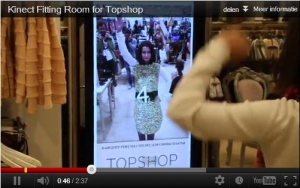
Kinect Virtual Fashion – by MicroSoft. It uses MS Kinect / XBOX to measure up your body, and then you can dress up virtually. On Youtube: http://www.youtube.com/watch?v=s0Fn6PyfJ0I
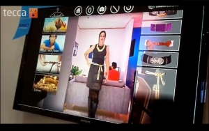
Cisco StyleMe Virtual Fashion Mirror, does about the same in retail environments, it’s a shopping business product
ImageTwin, http://www.imagetwin.com/ – use Kinect to obtain your body shape.
TC2, www.tc2.com – the guys behind the body scan technology

Now, given the body scan thing, where do you think that Virtual Fashion clothing comes from, since Javier Reyes teamed up with MicroSoft in various fashion conferences, and the software disappeared from the consumers software market in 2009?

Conclusion?

Now perhaps we can appreciate why FireFly is not that good in raytracing, and is very unlikely to become so in the near future. Till then we have to manage with translators (like Pose2Lux, or a Reality plugin for Poser perhaps?) into third party raytracers like LuxRender.

We also can appreciate why Cloth Room is very unlikely to undergo any drastic transformations. Till then we have to manage with a decent understanding of the tools at hand.

We also can appreciate why DAZ is demonstrating that Poser-compatibility is not an industry standard any more.

And finally, let’s not point at Smith Micro for the things they just inherited a few years ago.

Dynamics IV – 3 Cloth Simulation in Perspective

When I started to Google on cloth simulation, I stumbled into
http://www.animares.com/book/Secondary-Motion/Cloth/Hintergrund.html.
Its in German, on issues with cloth simulation. The page mainly noted to watch out for parameter settings, conversion and scale.
In short, if the parameters are determined for seconds, meters, kilograms etc and the mesh is defined in inches or internal (poser) units, then you’re off. I’ll let this alone, the Poser parameters are in semi-metrics (cm, s, gram), and I already mentioned the gravity matching the Earth surface conditions. Every now and then in this tutorial you’ll see me juggle to end up right. But for users of Imperial units (inches etc) there is a health warning in here: watch your units.
Also, cloth in real life does not scale, and neither do cloth simulators. Sheets of 1×1 mm, 1×1 mtr and 1×1 km really do behave different. Thread thickness plays a role, and so does the thread pulling strength and loads. You cannot fold the 1x1mm piece, and a 1km fibre will break under its own weight. Things like that.

The webpage also noted that although regular meshes do fine in most areas of 3D, cloth simulation is not one of them. Cloth Simulation benefits from a “Delaunay-Method” which gives irregular triangulation of meshes. It’s implemented in Sim Cloth / Clothmesh, in Cloth Reyes / Hexamesh, in ClothFX / Cloth Panel and in Maya / Cloth. So they said. A familiar collection.

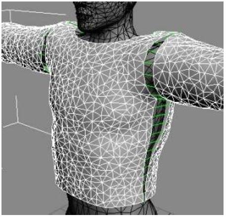
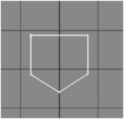
Since ClothFX ended up in 3DSMax (see Poser features in perspective) it’s the Hair&Cloth chapter from 3DSMax that presents clear examples. With a few splines the contours of a garment are defined, and the Garment Maker creates the irregular mesh from it. For a shirt in development:

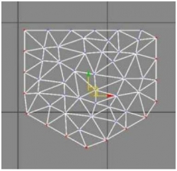
And for a pocket attached to it (just to illustrate what an irregular mesh looks like):

Since ClothReyes is implemented as Poser Cloth Room, let’s see what we can find out. Google is our friend.
Well, I end up at a program called Virtual Fashion (Pro 1.5), available in Spanish and English, July 2009, with the ability to export Quad and Hexa Meshes to Poser. Doesn’t it sound familiar (Poser features in perspective)?
A Mesh/Garment Maker apparently was not included when Cloth:Reyes was included into Poser, I can’t see it different. Poser got the simulator only.
In the meantime, Hexamesh itself is a toolkit doing fine in CAD/CAM environments, like the fabrication of (e.g. medical) components – which is not on our route.

I’m presenting this meshing story, because simulation results appear to be dependent on mesh structures and people ask (in forums etc) about “best mesh structures” and “what to do with existing mesh files”. We don’t need to re-invent wheels here. At least a serious part of this tutorial is devoted to mesh structures.
So I might need a tool to turn regular (quad, tri, …) meshes into irregular ones.

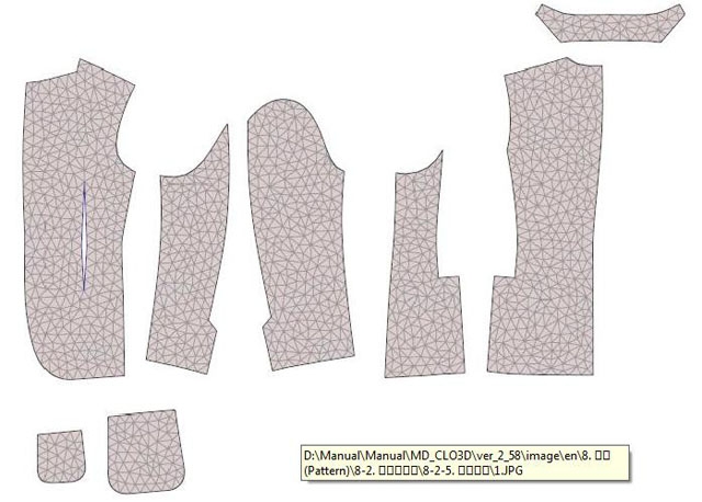
Since people are fond of Marvelous Designer as a cloth making toolkit, the Show Mesh example in the manual shows:

That’s not just simple triangles, that’s Delaunay Triangulation. Don’t look further!

I continued my strolling around the Net and in the end I found myself buried deep down in a worldwide scientific community on cloth simulation, US patents included, which evolved from about the mid ’80s. That was about the moment I stopped in the scientific arena after getting my MSc on applied math and experimental physics. I never looked back. This means to me that I will stop looking further into this area on the vertex level. Back to the front! Let’s make fun images. But I’ll give you what I found on the ways forth and back.

From www.poserfashion.net (before it got hacked, you can find the Original in Internet’s WayBackMachine) I learned that the author (Serge Marck) was into cloth sim long before Poser started doing it. He states that all cloth sim routines (those days) were based on the modeling of physical fibre behaviour in cloth. He also flagged and demonstrated that because of this modeling, the simulation results depend on non-virtual things as real world cloth size and structure. In effect, he showed differences (from Cloth Room) based on cloth size at constant vertex density, on vertex density at constant cloth size, and on mesh type (quad vs tris) at constant density and size.

His main source was a tutorial by P.S. Karthikeyan. It’s nowhere nowadays, I only could find a Russian translation of one chapter out of it (Google Translate is my friend too), on the modeling fundamentals. This said that all started in the ’80s from the well understood behaviour of cables (hanging bridges, telegraph cables) and the effects of fibre parameters, the effects of fibre thickness on those parameters, and the effects of gravity and wind. Cloth then is interpreted as a two-way weave of cloth fibres each described with cable behaviour.

It also said that – at those days – P.S. Karthikeyan was a 3rd year student on the Aerospace Institute in Madras, India. I did not find any other references to him related to cloth sim, after that. But I did find that the tutorial must have been very good, because it’s quoted in about every paper on this matter from those days on. Google rocks.

One of the papers I ran into looked worth downloading and sharing, it looked readable, an overview on fundamentals and implementations in the popular cloth sim software mentioned above and in various forumposts. Recommended.
This researchpaper can be downloaded here as well (10Mb, use Right-click Save As…), as it seems to be disappeared from its original location. This original location is the RISC – Research Institute for Symbolic Computation, deep down the science dungeons. Get me out!

With respect to all of this, Cloth Room definitely is a different beast than Materials Room or alike. It’s not a Room at all, it’s the Magic Kingdom Castle, or the complete Disneyland Park around it. I’m going back to the front gate. See you there.

Dynamics V – 1 Crash Course on Math and Physics

Understanding cloth and having a mental model of the physics involved is necessary but not sufficient to make effective and efficient simulating systems. Creating those systems is a world in its own right. Especially those with an engineer’s way of looking at things might be interested in this mini tour through the deep down dungeons. Crash Course on Math & Physics (this page) and Crash Course on Sims & Settings (next)really are the math and physics loaded chapters. Any use of the underground escape tunnel brings you into Muppets Lab “where the future is made today”. You have been warned.

Download this tutorial in PDF format (0.4 Mb).

Some people immediately zap away when they see even a two-character formula coming along, others insist in getting the rough engineering treatment to enhance their understanding. This chapter is for the latter part of the audience, although I can recommend the conclusions to everyone.

I’ll start with some math first because 1) it simplifies handling the formulas and 2) in the forums people have stated to have some issues handling and grasping it. Second I’ll do the physics, from an electrical point of view. This gives the proper resulting formulas in an easy way, but it’s too far away from our actual simulations. So third, I’ll present the physics from a mechanical point of view. Similar formulas but much closer to our actual cloth simulation.

Then, fourth, I’ll consider the simulation algorithms themselves. Finally, I’ll present some conclusions that help you further in handling the Poser parameters and cloth simulation.

Complex Calculations

In order to handle straightforward object motion, steady currents and flows, I can simply deal with real numbers. But handling disruptions, oscillations, alternating current and more becomes a lot easier when I extent my repertoire to imaginary and complex numbers.
In that area, the magic bullet is called ‘i’ with the property i² = -1. I don’t have to understand it, it’s there, period. Multiplying a real number b by i turns it into the imaginary i*b (or: ib for short), and repeating the operation turns it into i*i*b = i²b = -b which brings me back into the real world again. When I mix a real number a and an imaginary ib I get a complex number a+ib, and I can do all adding and subtraction while keeping the real and imaginary worlds separate:
(a+ib) + (c+id) = (a+c) + i(b+d).
Like I can represent real numbers on a straight line, I can represent complex numbers in a simple plane. I can use dots or arrows to them, and adding and subtraction behave like simple adding and subtracting those arrows as in vector algebra.

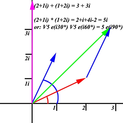
Complex numbers however are not very friendly in multiplication and handling powers, exponentials and logarithms. As you can see in
(a+ib)*(c+id) = ac + ibc + iad + i²bd = (ac-bd) +i(bc+ad)
real and imaginary parts of the numbers get mixed, which might turn longer calculations into a sheer mess.

The vector approach however gives us an alternative. Instead of considering the x and y components of the vector, we can consider its length R and angle q with the horizontal axis. This makes a+ib equivalent to R*[cos(q)+isin(q)]. Adding and subtracting from this approach becomes a nightmare, but multiplication, division and more becomes easy. Multiplication is: multiply the lengths and add the angles, which follows in a straightforward way from classic geometry (I’ll save you the details).

To simplify our tool even more, I use natural exponents and logarithms to rewrite R to e^r (or r=ln(R) ), and especially (cos(q) + isin(q)) to e^iq. In other words, a+ib becomes e^(r+iq) where r=ln(sqrt(a²+b²)) and q= arctan(b/a). This is handy, since multiplication of values is equivalent to the addition of exponents, and taking powers is equivalent to multiplying exponents, so (e^(r+iq) * e^(s+it) => e^{[(r+s)+i(q+t)]} and [a+ib]^N => [e^(r+iq)] ^N => e^N(r+iq).

So, with this dirty trick, the issues of complex multiplication and power-lifting are reduced to addition and simple multiplication. That’s a gain.

This is the basic tool, now the application of it in physics. Alternating currents, oscillating movements and the like can be described as x(t) = Rcos(wt) where R is the amplitude, and w=2 pi f, for oscillating frequency f. Each time wt makes a multiple of 2 pi, or each time ft makes a whole number, the oscillation starts anew. Now it has become a small step to state that the oscillation we see is just the real world part of a complex movement, which also has an imaginary component in a world we can or cannot imagine J.
But as a whole, its described with x(t) = Re^iwt or even with x(t) = e^(r+iwt).

The main reason for doing this, is that we need time-derivatives (and integrals) like dx/dt to get speed, acceleration and more. But the classical approach presents us a plethora of sine and cosine functions, and we really need a lot of geometry to get understandable results. In the new approach, we don’t.

When x(t) = e^(r+iwt) then dx/dt = iw * e^(r+iwt), so d2x/dt2 = -w2 * e^(r+iwt), from position to velocity to acceleration,
but also ∫xdt = 1/iw e^(r+iwt) and so ∫∫xdt2 = -1/w2 e^(r+iwt), from acceleration to velocity to position.

Going Electrical

In abstraction, basic physics considers a ‘field’ and a ‘thing’, and moving the thing against the field requires energy (from us or from the thing itself), while moving the thing along the field returns that energy back. One unit of field times one unit of thing make 1 Joule of energy, and if I do so every second it requires or generates 1 Joule per second or: 1 Watt of power.

Less abstract, in electricity the ‘field’ is electric potential (char: V) determined in Volt and the ‘thing’ is electrical charge (char: Q) determined in Coulomb. When such an amount of charge passes a measuring point within 1 second, we’ve got an electrical current of 1 Coulomb per second, or: 1 Ampere.
When I move such a charge to a place with a 1 Volt higher potential it requires 1 Joule (char: E, in formula: E=V*Q), and when I do so every second it requires a power of 1 Watt (char W, in formula: W = V*I). Especially this last formula on electrical power might hang somewhere in your memory, resulting from a physics class or so.

When I move a charge from one place to another, bridging a potential, it becomes harder for the next portion of charge to do the same. The source of the charges becomes short due to the displacement, or: anti-charged and as we know opposite charges pull each other. The destination of the charges gets a surplus or: gets charged, and similar charges push each other. In other words, by moving a charge across a field, it gets less interesting to continue, the field itself gets reduced. The ratio between these is understood as: electrical capacity (char C, measured in Farad).
In formula: dQ = C dV, when I move a charge dQ the field changes dV. When the device that includes the source and the destination of the charge is said to have a large capacity, this means that the displacement of large charges have little effect on the field.

Even when moving the charges hardly effects the field, the charge elements (e.g. electrons) have to bridge the gap between source and destination, collide to each other and to loads of molecules in between, and dissipate some heat. This is understood as electrical resistance (char R, measured in Ohm).
In formula: V = I*R or I=V/R, Ohm’s law. A large resistance is like having air (or less) between two poles of a battery, they are electrically isolated, there is hardly any current and no energy loss. A small resistance is like short-circuiting the battery with a copper wire. Lots of current, and the heat might even melt the wire. As current I = dQ/dt we see that first we had a relationship between ‘field’ V and ‘thing’ Q, and now we’ve got a relationship between V and the first time-derivate of the ‘thing’: dQ/dt.

So the next step is to investigate what happens with that second time-derivative, or: dI/dt. This just means: alternating current. When alternating current is applied onto a coil, it generates an electric field. This is understood as electrical induction, the fundament under dynamos, generators, turbines and the like. Char: F (after Faraday), measured in Henry (both did the discoveries at the same time).
In formula: V = F*dI/dt or dI/dt = V / F, a large induction generates a strong field from the alternating current.

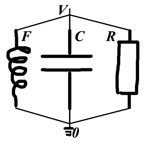
Now, let me bring all the elements together. I’ve got a device with two poles, I apply an alternating voltage onto the poles, and the charges and currents in the device start working in parallel:

Working in parallel implies that I have to add the individual currents, so: (I1+I2+I3) = I total = Voltage / “Impedance” (Impedance is some kind of resistance for alternating currents and voltages, taking capacity and induction into account).

Alt. Voltage Vexp^{iwt}
Capacity I = dQ/dt = C * iw * Vexp^{iwt}
Resistance I = 1/R * Vexp^{iwt}
Induction I = 1/F * 1/iw * Vexp^{iwt}
In parallel I = [ C * iw + 1/R + 1/F*1/iw ] * Vexp^{iwt} = 1/IMP * Vexp^{iwt}
So IMP = 1/[ iwC + 1/R + 1/iwF ], after taking the inverse on both sides
= iwR / [-w2 RC + iw + R/F], after multiplying with iwR on both sides
= iwR [ (R/F-w2RC) – iw]/[ (R/F-w2RC)2 + w2], after multiplying with [ (R/F-w2RC) – iw]
= w * [w/R + i (1/F-w2C)] / [(1/F-w2C)2 +(w/R)2]
If R very small (short circuit), then 1/R becomes dominant and IMP => (w2/R) / (w2/R2) = R2/R = R
If R very large (isolation), then IMP = iw / (1/F-w2C) and becomes quite large when 1/F-w2C => 0,
that is: w2 => 1/FC. Then the impedance => R again.
This w = sqrt(1/FC) represents the resonance frequency of the system, it behaves at a minimal energy loss.

Now we’ve got the essential formula, let’s apply them on a mechanical system.

Going Mechanical

The mechanical route follows the same approach. The ‘field’ is force (char F, measured in Newton) and the ‘thing’ is displacement (say X, measured in meter). Applying a force of 1 N over 1 m requires 1 J of energy, and applying that force over a route with a speed of 1 m/s requires 1 W of power. Note the similarities with electrical.

A spring pulls and pushes, proportional to its stretch: F = S * X. The stronger the spring, the more force is required to stretch it (with the same amount of displacement). Spring strength does not have a specific name, it’s measured in N/m.
Spring strength is not related to any mass, but when a mass is attached to a string, the force will generate an appropriate acceleration: F = M * a, Newtons Law, where a is d² X/dt², the second time derivative of the ‘thing’ we’re considering. M is mass, in kilograms.
So we’ve seen forces proportional to distance X (the spring) and to its second time-derivative acceleration A (gravity like). So all we need to make it like electrical, is a force that is proportional to the first time-derivative of distance, which is: speed, or velocity v. This introduces: damping D as in F = -D*v. The faster you move, the more the force will work against you. Air-resistance is one example of them.
Now we can make the step from electrical to mechanical, just by substituting the equivalent concepts
- So electrical capacity C relates to 1/S spring strength
- So electrical resistance R relates to 1/D damping
- So electrical induction F relates to M mass
And so w = sqrt(S/M) represents the resonance frequency of the system. The resonance becomes noticeable when there is only little damping. Strong springs with little mass with make high frequencies, loosening the springs and/or raising the mass will reduce the resonance frequency. Damping will kill the oscillations and will produce a stable result faster.

RESULT: IMP = w * [wD + i (1/M-w²/S)] / [(1/M-w²/S)² +(wD)2], times S²M² at both sides:
= wSM * [wDSM + i(S-w²M) ] / [(S-w²M)² + (wDSM)²]
=> 1/D at the resonance frequency w = sqrt(S/M)

Mechanical systems and electrical systems do compare, but to a certain extent. Electrical components can be made quite ideal: capacitors with a good isolation and no leakage (extreme resistance), resistors with hardly capacity or induction by their own, inductors with metal kernels and so on. And those systems are pretty linear over a large range of values, from electron beams in a CRT monitor to outdoor flashes in a thunder storm, the same laws keep applying.

Mechanical components are far less ideal: springs do have mass and damping by themselves, and the stretching is far from linear. When the spring is made of an iron wire coil, there are upper and lower limits to its expansion or compression depending on the length and thickness of the wire used. So in fact the formula should read F = S₀ X + S₁ X³ + S₂ X⁵ + …

Odd powers only, as all forces work in one direction: against the displacement.
The same holds for damping, as can be found in any aero/fluid-dynamics class or textbook. For low speeds it’s proportional, but at higher speeds the additional terms kick in quickly: F = D₀ X + D₁ X³ + …

All this means that the math still can be done but that the final resulting formulas become longer and less friendly.

Conclusions

By looking at complex numbers in addition to normal, real numbers, I got tools for expressing fluctuations in a more elegant way. By applying them to electrical circuits with alternating current, I got the formulas for the “impedance” of a system responding to alternating inputs. By applying those formulas to a mechanical context, I got a descriptor for a mechanical system, responding to external forces.

I found that such a system is characterized by

Mass (M), making it harder for a force to accelerate an object
Damping (D), making it easier for a force to reduce an objects speed, and making the object lose energy faster
Spring Strength (S), making it harder for a force to displace an object
Resonance, the tendency to vibrate with a frequency sqrt(S/M). This is reduced by Damping.

Dynamics V – 2 Crash Course on Sims and Settings

Understanding cloth and having a mental model of the physics involved is necessary but not sufficient to make effective and efficient simulating systems. Creating those systems is a world in its own right. Especially those with an engineer’s way of looking at things might be interested in this mini tour through the deep down dungeons. Crash Course on Math & Physics (previous page) and Crash Course on Sims & settings (this one) really are the math and physics loaded chapters. Any use of the underground escape tunnel brings you into Muppets Lab “where the future is made today”. You have been warned.

In this chapter, I’ll consider the simulation algorithms themselves. Finally, I’ll present some conclusions that help you further in handling the Poser parameters and cloth simulation.

Going Sim

Creating a computer simulation of a mechanical system requires the build of a ball-and-spring network. Like a mesh, the vertexes are small balls with carry all the mass, while the edges connecting the vertices are small (mass-less) springs which do the pushing and pulling. Balls and springs both take their share in damping, and the balls pick up the external forces and limitations like gravity, attached weights, air-damping, collision and friction to objects.

In order to make the simulation work like the real thing, various technical (constructive) aspects require attention. Building goods simulations is a serious profession. To name a few:

Resonance
mentioned already as a ‘natural aspect’ of electrical and mechanical circuits. What does it do?
Say, the resonance frequency is: 100. This means that a vertex is oscillating around its proper place to be, at 100 times a second, real world time (as the values for Damping, Spring strength, Mass, Object size etc. are real world values). If the simulation recalculates the positions of the vertices in steps of 1/1000 of a second, the oscillation would be clearly visible: a predictable instability. The oscillation is samples ten times a period.
If the simulation recalculates the vertex position each 1/60 of a second, the neat oscillation would appear as a random jumping around, as a noise, an unpredictable instability. The oscillation is samples less than once a period.
In all cases, an instability which makes that the sim needs longer calculation times to arrive at a steady result. In other words; we have to wait till the oscillation-energy is faded away. The best way to speed that up, is to increase the damping, as this stands for energy loss per second.
Mesh density
in how many subparts do I chop the system? In cloth, which can be considered a surface, halving sizes in two dimensions imply quadrupling the amount of balls and springs, and calculation time. In Poser I’ve seen pieces of cloth chopped into pieces of 5x5cm (divides 1 m² into 400 balls) to 1x1cm (10.000 balls), but a cotton fibre is as thin as 0.1mm (100 million balls per m²) and no one is building a sim like that. But by not doing so, one runs the risk of “finite element artifacts”.
Non linearity
as long as the mechanics, the systems and the forces considered are linear, increasing mesh density has no effect. For instance, the cloth has a mass density of 1kg/m2, and whether I chop it into 10.000 or 100 million balls will not have effect on the effects of gravity or air damping on the cloth. And when the cloth is 1 m x 1 m and I chop 1 horizontal fibre into 100 little springs, or 10.000, will not have effect on its sheer stretching behavior. But when things are non-linear, mesh density makes a difference.
- Resonance.
  as discussed in the electrical and mechanical sections, each system has some kind of resonance frequency for which the damping is minimal. If I give the system a kickstart, it will send all sorts of signals around in all sorts of frequencies (noise like) but the resonance one stays alive the longest. For mechanics, it’s proportional to sqrt(S/M) for spring strength (say: stretch resistance) S and mass M.
  Now I chop the cloth into pieces, at mesh density d. For instance, d=100 chops the 1x1m cloth into fibers of 1 cm (with stretch resistance S/100) and pieces of 1x1cm (with mass M/10.000).
  As a result, the resonance frequency goes up a tenfold (sqrt(d) to be precise). As stated above, this affects the noisiness, the randomness of the vertex positions.
- Folding
  one can imagine that making an angle between two adjacent polys in a mesh is easy for very small distortions but becomes quite hard for the larger angles. Each extra degree of bending requires more and more force to accomplish. So if the 1x1m cloth is divided into 10x10cm pieces and I need a 30° between two adjacent pieces, or the cloth is divided into 1×1 cm pieces and I need 3° between two adjacent pieces but for 10 pieces in a row, the latter requires less force to accomplish.
  In Poser terms: with the same fold-resistance, finer meshes will fold easier. Mesh density makes a difference.
Edge effects

You might have experienced it when making waves with a heavy rope or garden hose (if not, give it a try). When the other end is loose it jumps up end down wildly. Actually, when your waves in the rope have some amplitude, the loose end will show you the double. You can create some constant wave in the rope if you manage to pick a frequency that creates a specific length of the wave: such that there are ¼ , ¾ , 1 ¼ etc waves in the length of the rope.
When you fix the other end, to a wall or a pole, the other end will be still at any time. You can still make those standing waves but at different frequencies, such that there are ½, 1, 1 ½ etc waves in the length of the rope.
Not only ropes and garden hoses, but simulations as well suffer from edge effects. At the end of the ball/spring network, balls have less springs attached. Does that require heavier balls, more strength for the remaining springs attached to those balls, or just the other way around? Does the sim require fixation (like the rope at the wall) or does it allow for jumping around (like the open end case)?
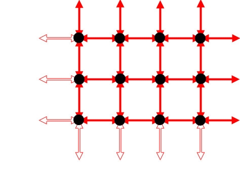
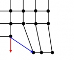
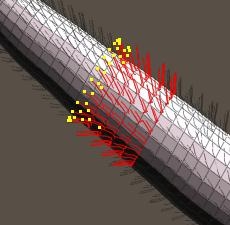
Anyway, as the image illustrates, the vertices at the edge of a mesh behave different because they are missing forces, as the springs (in between edges) are not there.
All this is up to the sim builder, and there is no real escape. No sims without edge effects, unless one can make calculations on an edgeless world (a globe, e.g.). For cloth and clothes, one might give the edges specific treatment, like is done with real clothes. A rim, with higher mass / density, less stretching and less folding.
Calculation order
There are various ways to get the results of a simulation. Iterating step by step is always required, but one can take a ball/spring network in iteration N, and use that information only to calculate the next iteration N+1. A layered approach, so to speak. Another, more continuous approach, is to take a vertex with the information from iteration N, plus the already derived information for surrounding vertices from iteration N+1, and calculate the iteration N+1 for that vertex.
Again, this is up to the sim builder and there is no escape. The first approach requires more memory (as two nets have to be kept in store) and requires more iterations (as less info is used per step), but is easier to implement as a multi-threaded routine, it will be less prone to edge effects, and if any these will be distributed quite evenly along all edges. The second approach requires less resources, less iterations, but is typically a single-thread routine which will add directional effects to the edges. That is; it will calculate the vertices in a specific order, like top to bottom left to right so edge effects will typically appear in the top left or bottom right corner.

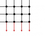
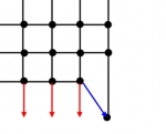
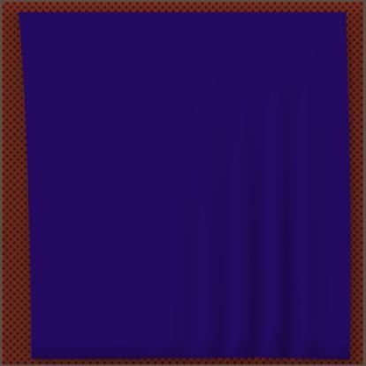
First, there is gravity only. But having the first ball moved will skew the forces on the second, and so on.

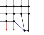
Then, you will get this, a piece of cloth skewing to the right-bottom corner when let loose.

I suspect modern simulators like Marvellous Designer to be of the first kind, and Poser Cloth Sim of the second kind as it stems from the Poser 5 period (even before) and has hardly seen a methodical update after then.

Unsimulated aspects
Aspects of cloth which are absent in the sim, are: thread thickness, and weave density. Thicker threads make thicker cloth, with more weight per square inch, are harder to fold especially over large angles, are harder to stretch, and might increase the friction between threads. This friction between threads by itself affects shear and folding, affects air damping, and so on. A high weave density (threads x thickness per stretching meter) has similar effects.
Modern advanced cloth simulations take threads and weave aspects into account. Poser cloth room limits itself to global cloth descriptors which include named details. From that, Poser simulates non-woven materials as well; leather, fleece, rubber and the like. This implies a simulation mechanism which is further away from physical details in the real world.

Perhaps you’re familiar with software creation. Then you’re aware that only 20% of the effort really goes to the program’s functionality, and 80% is about the user interface, preventing people from inputting erroneous values or clicking buttons at the wrong moment or selecting impossible combinations of options; that is: making the software user aware. For sims, things are about similar. 20% is about the simulation itself and 80% is about handling the resource requirements, the artifacts from resonance and edges and non-linearities of nature.
This implies that you might have to upgrade yourself from a Poser User to a Poser Sim User.

Going Poser Cloth Room

Offering a cloth simulator to end users introduces a guaranteed set of shortcomings which are not well understood, by those users at least. Not simulating various aspects of cloth (thread thickness, weave density, weave structure) makes it harder to translate the real world to sim parameters, and impatience combined with insufficient resources introduces algorithms with additional artifacts (like skewing cloth).

Mesh structures, mesh densities and various resistance and damping settings will affect the presence or absence of edge effects and resonance, which – at least from an end users perspective – introduce seemingly random vertex movements and floppy edges. Increasing mesh densities, resistance and damping as well as longer simulation times (more frames) kill those effects eventually. Sometimes raising the damping might just make things worse instead of better. But for most people it’s unclear that they have to cope with simulation artifacts that have nothing to do with cloth behavior or with their use of Cloth Room.

In the end, it’s clear not what is meant by the various kinds of parameters:

Resistance, against pulling or torque, is like electrical capacity: it stores energy in the cloth and releases it later on.
Damping is like electrical resistance: it turns cloth movements into energy loss and brings the system to a standstill.
Gravity, Friction and Wind make the forces (via Mass, or: Cloth Density), and so generate the energy for Resistance to store and for Damping to lose. Which effectively make these the drivers of the simulation.

Unsupported aspects

When I take the backdoor to enter the stage Cloth Room behind the scenes, that is: I take a look at the Python manual, I find some parameters which go unsupported by the properties dials in the 4^th panel of the cloth room. These are all of them:

Airdamping Dial: Air Damping
Clothclothforce always 10, no way to set it manuall (python script required), unclear what is does
Clothfriction Dial: Cloth Self Friction
Dampingstretch Dial: Stretch Damping
Density Dial: Cloth Density (grams per cm2, 1g/cm2 = 10kg/m2)
DynamicFriction Dial: Dynamic Friction
FrictionFromSolid Checkbox: Collision Friction. If checked, the Object parameter are used instead of the Cloth parameters. So either cloth shows a different behavior over rough and smooth object surfaces but the same for all cloth elements, OR cloth shows a different behavior for various cloth elements but the same for all collision objects. In one sim one cannot have both, various cloth elements over various surfaces.
FrictionvelocityCutoff always 30 (cm/s), no Dynamic Friction below this speed, no way to set it manually
ShearResistance Dial: Shear Resistance
SpringResistance no way to set it manually, might be related to EdgeSprings, which are OFF (0)
StaticFriction Dial: Static Friction
Thickness is derived from Collision Depth and Collision Offset, which define distances between the outside of the object and the outside of the cloth, which are the parts we see. These collision parameters BTW are aspects of the objects, not of the cloth so in one sim all cloth elements have the same thickness for a specific object, and another thickness or another object. So Cloth Thickness is not very well represented. I guess it doesn’t do anything
U-BendRate not used, no way to set it manually
U-BendResistance Dial: Fold Resistance
U-Scale purpose is unclear, no way to set it manually
UseEdgeSprings 0/1 whether to use Edge Springs calculations. No way to set it, though. It’s OFF (0). Here you have the ability of Cloth Room to manage edge effects, as discussed in earlier chapters.
U-StretchResistance Dial: Stretch Resistance
V-Bendrate V-values are not used
V-BendResistance ditto
V-Scale ditto
V-StretchResistance ditto

File layout

Cloth info about a cloth prop or cloth figure is stored in the pp2/ppz (prop) and cr2/crz (figure) respectively, and looks like:


    vertsGroup _default_
        {
        v 0 
        v 1 
        … 
        v 6003 
        v 6004 
        stitchVertsGroupProperties 
            { 
            U_Bend_Resistance 30.000000 
            V_Bend_Resistance 5.000000            \ no dial 
            U_Stretch_Resistance 40.000000 
            V_Stretch_Resistance 50.000000        \ no dial 
            Shear_Resistance 50.000000 
            U_Scale 1.000000                \ no dial 
            V_Scale 1.000000                \ no dial 
            Density 0.010000 
            Thickness 0.000000                \ no dial 
            Spring_Resistance 5000.000000 
            Air_Damping 0.020000 
            Dynamic_Friction 0.100000 
            Static_Friction 0.500000 
            Friction_Velocity_Cutoff 30.000000    \ no dial 
            Cloth_Cloth_Force 10.000000        \ no dial 
            U_Bend_Rate 0.000000            \ no dial 
            V_Bend_Rate 0.000000            \ no dial 
            Cloth_Cloth_Friction 0.000000 
            Damping_Stretch 0.010000 
            get_friction_from_solid 0 
            Use_Edge_Springs 0                \ no setting 
            anisotropic 0                    \ no setting 
            } 
        } 
    vertsGroup _choreographed_ 
        { 
        } 
    vertsGroup _constrained_ 
        { 
        v 3 
        v 6 
        … 
        v 5752 
        v 5753 
        } 
    vertsGroup _softDecorated_ 
        { 
        } 
    vertsGroup _rigidDecorated 
        { 
        }

CaseStudy: Hairy Stuff (1 Intro)

As long as your hair is styled properly …

Download this tutorial in PDF format (2.0 Mb).

Introduction

This Case Study is a beginners guide into Poser Hair Room, and will be about assigning fur or short hair to objects, clothes and animals and about assigning facial and body hair to humans.
To deploy the basic techniques I’ll put fur on a purse and on a jacket, and play a bit with hair coloring.

Then we’ll have a look at a pre-made, commercial product: Snow Bride. After that, I’ll consider more elaborate figures like a toon kitten or puppy and investigate under water scenes by considering a long-haired fish as well. Long hair on animals brings up horse manes and tail, so I’ll give that some attention too. The step to humans is a small one then, as long as I start with facial and body hair.

Long hair on human heads will be dealt with in #Photo Shoot#. Have a good hairday.

CaseStudy: Hairy Stuff (2 Purse)

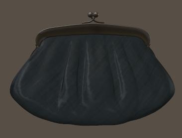
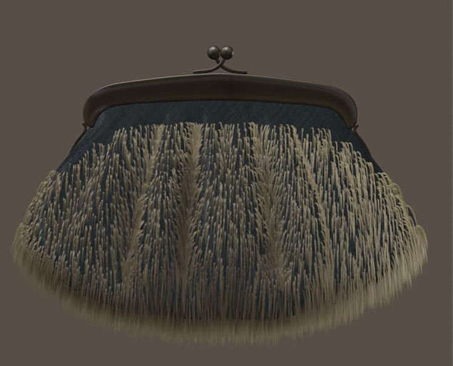
In this chapter I’ll put fur on a simple ladies purse (from the Noctia outfit).

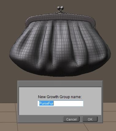
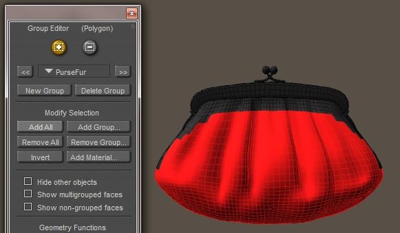
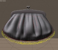
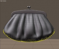
I switch the preview to Smooth Lined (or Flat Lined) to see the polygons, open the Hair Room, ensure I’ve got the Purse figure as well as the Purse bodypart of it selected, I click [New Growth Group] in panel 1 and assign “PurseFur” as the name for the new hairdo.

In order to select the entire surface into my hair group, I click [Edit Growth Group] which opens the Group Editor, and [Add All] adds all polys from the Purse\Purse (=figure\part) to the hair group.

The option Hide Other Objects helps me to concentrate on the Purse object, and when I check Show Multigrouped faces I get the entire purse, as all polygons are part of the group Purse as well as part of the group PurseFur.

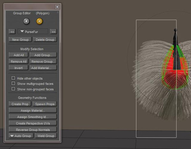
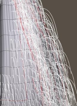
For more details on the Group Editor, just consult the Poser Reference Manual. I can close the editor now, and click [Grow Guide Hairs] in panel 2.

Now I realize that I don’t need hairs on the back, I’m only going to render the front side. So I [Edit Growth Group] again, tick the [-] option to subtract faces from the group, position the camera so I can view the purse from aside. While selecting polygons or just clicking them, and by clicking [Grow Guide Hairs] regularly, I can check when I’ve got the proper surface. If I see any hair growing out of unwanted places, I still have to deselect a poly.

Growing Hair
Next, I estimate the purse at about 20cm wide and 10cm high, that makes 200cm2. When the fur comes from an animal with a dense coat I guess I’ll need 400 hairs per cm2 (human heads do about 200), so that will be 80.000 hairs. In this tut, I’ll far less. Given the size of the purse, the hairs can be 1-2cm long, and 1-2mm thick as animal hair. These short, thick hairs covering the purse are not going wild in wind, gravity or any styling so I do not need high mesh resolutions.

So on panel 2: Hair Length = 0,015 and Length Variance = 0,005 (my Poser is set to Meter units, for inch-units you can use about 0,6 and 0,2 respectively). On panel 3: Hair Density = 400,000, Tip Width=1, Root Width=2, Verts per Hair=4. For clarity, I zero out all other parameters in panels 2 and 3 (Kink Scale has a minimum of 1).

Important note: Hair Length and Variance are presented in user units, in my case: meters. My 0.015m = 1.5cm = 0.6″. Hair Density is presented in (hairs per) square user units, in my case: hairs per m2. My 400,000/m2 = 40 /cm2 = 258/inch2.

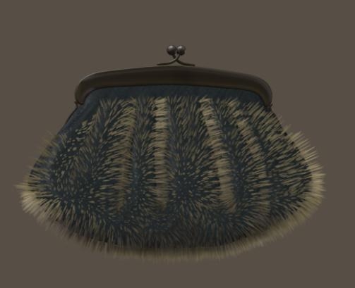
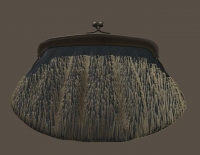
As all hairs are standing straight out, as I haven’t done anything dynamic and as there is a serious color contrast between the purse and the hairs, the rendered result looks like a porcupine. But I’m not done yet.

Since animal fur grows quite flat onto the skin, I can use the Pull Down dial to establish that effect. There is nothing to Pull back or Pull Side, so I leave these alone (at 0.0).

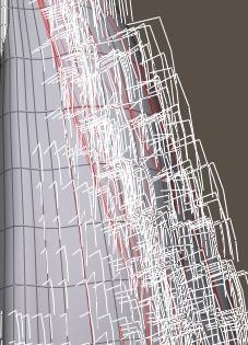
As the left image (shot from aside) reveals, I need a large value (0.005) and the hairs bend quite sharp. This is due to the lack of resolution, a hair can only bend at a vertex. So I turn the 4 Verts per hair up to 32. And now I get a much smoother result, at a much lower value (0,00004) – right image. And as I don’t need clumpiness or kinks in this straight animal fur, I decide that this should do.

From this I can identify some areas for improvement.

The hairs are the bottom should be shortened (shaved).
I need a coloring of the purse and the hair, and blend them together
If then still needed, I might need a higher hair density. This is simply a matter of raising the value and turning the appropriate dial. Twofold, Fourfold, I’ll see.

Shaving
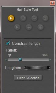
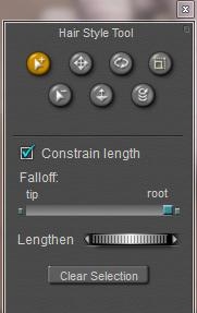
Of course I can remove the bottom area from the PurseFur hair group, and create a new one with shorter hairs. But now I’m going to alter individual hairs instead, and so I click [Style Hairs…] in panel 3. The Select+ option is on by default, and I start selecting all hair(tips) that I want to alter.

Then I use the Lengthen dial (rotate left) to shrink the selected hairs. When done I [Clear Selection], spot any hairs I missed and give them the same treatment.

Notes:

There is no way to save selections for later use. Once done, I’ve got to reselect them.
Any touching of button, dial of value field in panel 2 will completely undo all styling for all hairs in the hair group at hand. This means that I must be sure about Length and Pull settings before starting to style.

Dye Hair
In order to change to coloring of the purse and the fur, I step into Material Room, Advanced tab, and select the PurseFur prop from the objects list. This prop contains all hairs in that group, but not the purse surface itself.

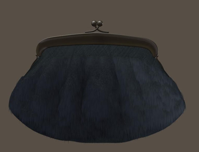
The fur material is set to its Blonde default, and the first thing to do is to increase the Root Softness. This blends the root of the hair into the surface by making the hair increasingly transparent from the outside in. But in this case, the contrast between haircolor and surface color is so strong that I really need recoloring. Since the purse is dark teal/blue-green I selected Root = RGB(31,33,32), Tip = RGB(71,85,99) and Specularity somewhat in between, and set Root Softness to 0.5.

The result was not that satisfying, so I severely reduced the Specularity (and Alt_Specularity) of the purse itself, but reducing the brightness or their color swatches. And – as stated in the improvement notes above – I drastically increased haircount at the cost of longer render times and higher memory consumption. From 400,000 to 1,280,000.

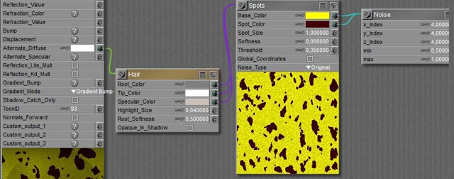
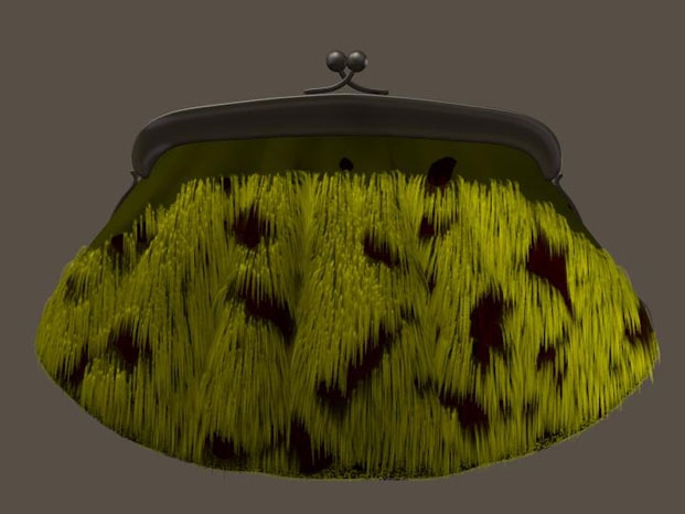
To have more fun, I turned the purse into Marsupilami, the comic animal by Franquin (www.marsupilami.com).

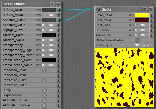
So I altered the material for the purse itself into a simple one.

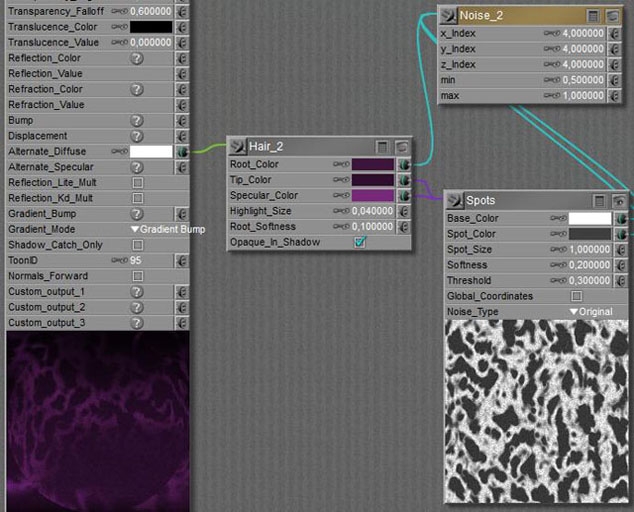
And I copied the Spots into the material of the PurseFur object, in between the original Noise and Hair nodes.

Since I’m using the same Spots in all places, any differences come from the filtering by the colorswatches. The Diffuse and Specular in the purse material itself both are the darkest, while Specular has a reduced value (0.1) as well. Only metals have a high specularity. My idea on finished animal furs is that the skin itself has the darkest tone. In the PurseFur hair material, the Root color is the next darkest, the Tip color is just white and the specular for the hair is somewhat in between with a slight brownish hue. The effect of the (already present) Noise node is very visible in the spots now.

And since the hair matches the cloth of the purse, I can do with a reduced hair density. So I lowered it from 1,280,000 to 320,000, and got after rendering:

CaseStudy: Hairy Stuff (3 Jacket)

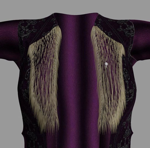
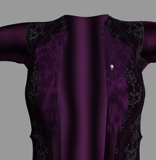
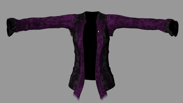
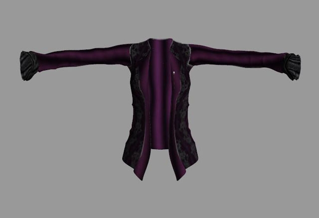
This is the jacket from the Witch Hunter for Vicky4.

It has some decorated parts on the sleeves and the front, and I’m going to “furrify” the smooth parts. This is not very different from handling the purse, but let’s look before we leap.

From a fur point of view, the jacket has a Left Sleeve with the hairs growing sideways (positive X, to our right), a Right Sleeve with the hair growing sideways (negative X, to our left) and a Body. Each of these is built from three mesh components:

Left Sleeve = Left Collar + Left Shoulder + Left Forearm
Right Sleeve = Right Collar + Right Shoulder + Right Forearm
Body = Hip + Abdomen + Chest

As I found out by clicking around on the jacket. In the Materials Room I found portions for

A Pen, that’s some jewelry sticking upon the left front of the jacket
Sleeves, that are the ultimate ends at the arms
Jacket, everything else

Each sleeve – from arm pit to wrist – measures about 50cm long x 40cm circumference = 200cm2, the body measures about 70cm high x 100cm circumference = 7,000cm2, minus 20% for the open front minus 20% for the decorated parts make say 4,000cm2. From the 7,000cm2, half of it sits at the back of the body, which leaves 4,000 – 3,500 = 500cm2 for the front side of the jacket. We’ll need this info to set the haircount to reasonable values.

Setup
I enter the Hair Room, select the Right Collar (mesh group / subobject / bodypart), start [New Growth Group], name it (“RightArm1” for instance), click [Edit Growth Group] to collect the polygons for the group, and just [Add All] to finish. Perhaps I’ll need to do some more detailing later on, but this gives me a start.

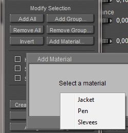
I select the Right Shoulder in preview, repeat the procedure (“RightArm2”, select Right ForeArm, repeat the procedure (“RightArm3”) but instead of using [Ad All] I click [Add Material], as I want to exclude the decorated ends. Those ends were assigned to a Sleeves material group, so I select this, and then click [Invert] because I just want the other part.

While the jacket has object-groups and material-groups which technically are independent, I must create hair-groups for each separate object-group, and I can use the material-groups for further selection within that object-group. Like above, Sleeves addressed both left and right end but while working on the right arm object, I could address the right part of the material group only.

And I cannot make one single “Right Arm” hair group, I end up with three parts. When I select the Right ForeArm in preview, then hairgroup RightArm3 is accessable only.

This way I also build my LeftArm1/2/3 hair groups, and also make my JackBody1/2/3 groups out of Hip, Abdomen and Chest. For defining JackBody1 from the Hip etcetera, I manually select the relevant portions as I’m avoiding the decorated parts and – for the moment – I don’t need hair on the back for my current renders.

Using the mouse for selections requires some practice. Adding, deleting and turning cameras is a must for the fine details. Sometimes it pays to make larger selections, and exclude (using the [-] option) some polys later. Some people might prefer a tablet for this kind of work.

Sometimes handling logic brings a way out. Excluding the Pin on the chest part could be done easily, by selecting the jacket part completely, then inverting (to everything but…), then adding all polys with the “Pen” material like I did with the Sleeves material before, and Inverting again.

Time to save now.

Growing fur
My next step is to grow fur on one area (say: Chest = JackBody3) , adjust it till I like it, and then (manually) copy my findings to the other areas. So I select that part of the jacket (preview), as well as the hairgroup (panel 1), and deploy panel 2 to [Grow Guide Hairs] with a length of 3.5cm, a Variance of 0.5cm (so: hairs will be 3-4 cm), no Pull back or Pull Side but a serious Pull Down supported by enough Verts per Hair. Kinks and Clumpiness could be zeroed out, and I vary the hairs between 2 (root) to 1 (tip) mm.

It renders like this:

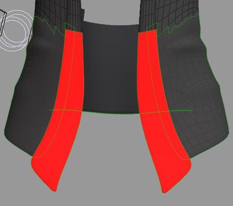
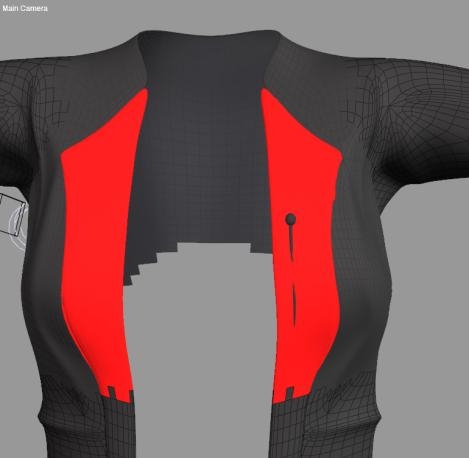
From this I learn that it’s better to exclude the polys from the hair groups that do not face the front, but face up, down or sideways instead. The hairs from the side do not contribute to a nice result.

When re-selecting the bodypart for re-editing, be sure that you’ve got the object part (here: Chest) and not the hair-prop JackBody3. The first one contains the Hair Growth Group including all settings, the second contains the (guide) hairs that result from that. Check Hide Other Objects in the group editor to get rid of the hairs while (re)selecting.

Then I need to color the hair, and I need to set the hair density to a proper value. The full front of the jacket was estimated 500cm2, so this third part might be 180cm2 and with 200 hairs/cm2 that makes 36,000 hairs. To be halved or doubled depending on coloring.

Handling the material
I selected the Root color to match the purple surface RGB=(60,20,60) while making spots of darker tips RGB=(30,10,30) and added the same spots to a bright specularity RGB=(120,40,120), all in the same hue.

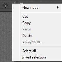
Once I like it, and once I’ve made another hair group, I can copy this material to the other hair groups:

With the triangle at the upper right corner: Select All
Copy
Then select any other hair Prop (the prop, not the growth group body part),
And with the same triangle-menu: Paste
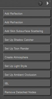
Then, from the list of buttons: [Remove Detached Nodes] to clear the original hair material
Select another hair prop, paste again, remove original nodes, and so on.

Details galore
Hair was quadrupled (144,000 for this area) and I’m still convinced that the top inner side, and the top outer side can use a shave. This is due to the high density of small polygons to make a smooth bend in the jackets form. With a guide hair per vertex, and populated hairs per guide hair, many small polygons mean: many hairs in that area.

Now I’ve got my settings I can do the other parts of the jacket.

Hair length 0,0350
Variance 0,0050
Pull 0,00012
Density (72.000 to 144.000)
Tip 1
Root 2
Verts 32

The arms have the hair pulled sideways instead of down, require far more pull and mind the +/- sign for the proper direction.

This still leaves room for perfection:

Around the Right and Left Collar or: RightArm1 / LeftArm1 elements, hair (polys) should be deleted and/or hairs should be shaved using the Hair Editor, and hair Pull and Density have to be looked into. Plus the details for shaving mentioned already for the upper/inner portions of the jacket. As usual, the devil is in the details, and so is our time.

CaseStudy: Hairy Stuff (4 Snow Bride)

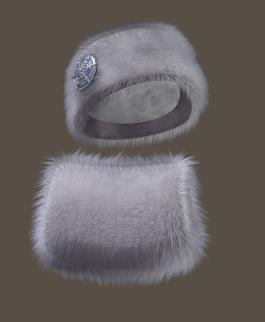
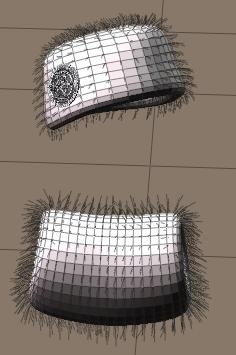
Snow Bride is a commercially available set of clothes for the well-known Vicky4 character. The clothes are fur, and look like this.

Let’s analyze the parameters, and learn from them.

Structure

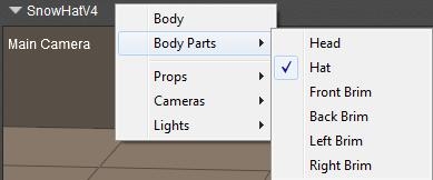
The hat as well as the muff have an Underfur as well as a Top-fur hair growth group, that’s four in total.

and The other object parts have no hair groups. This is found out by selecting each part of each object looking in panel 1 which tells me about the available hair groups.

Clicking [Edit Growth Group] tells me that the inner bands, and the medallion on the hat are neatly excluded from the groups.

Guide hairs

Switching the preview to Flat Lined or Lit Wireframe (Ctrl+5) reveals the 3D mesh geometry, and clearly shows 1 guide hair per vertex. Or better: two guide hairs in this case as the Underfur and Top-fur groups overlap, so each vertex is in two groups.

For each hair growth group selected in panel 1, I looked at panels 2 and 3 and noted the numbers. The three Pull parameters were 0,0 in all cases, and indeed all hairs grow right up from the surface.

&ndsp;	Hat-topfur	Hat-underfur	Muff-topfur	Muff-underfur
Polygon size	2,5×1,6=4cm2		1,4×1,4=2cm2
Nr of polygons	Ca 250		Ca 500
Hair length	0,030 cm	0,030	0,030	0,023
Length variance	0,000	0,000	0,015	0,011
Density (per cm2)	22000 (2.2)	88000 (8.8)	33000 (3.3)	88000 (8.8)
Tip width	0,4 mm
Root width	2,0 mm
Clumpiness	0,25	0,10	0,25	0,10
Kink Strength	3,0	7,0	3,0	7,0
Kink Scale	10,0	10,0	10,0	10,0
Kink Delay	0,1 (10%)	0,0	0,1 (10%)	0,0
Verts per hair	4	4	4	4

Analysis
Looking at the hat first, the hairs from both groups have equal length (3 cm) and no variance, are rather thick at the root and thin at the tips (typical for animal hair: thick roots for better protection, and thin tips due to natural wear and as they don’t do haircuts). The underfur is much denser (88 compared to 22 hairs per cm2. The hat measures 250 polys of 4cm2 each so the 88000 resp 22000 hair find their place at 1000cm2 hat). But even the total density of 88+22=110 is still half the coverage of the human head (about 200 hairs per cm2), which by itself is about half the coverage of real life animals.

So the objects have a furry impression, will need appropriate coloring of the cloth as well, but don’t resemble a full real animal coat. The underfur is denser, more even (the clumpiness of the topfur increases the furry impression) and more curly which makes is look denser. The topfur is not only less curly, the curls start somewhat (10%) away from the object surface.

The muff measures 500 polys x 2cm2 = 1000cm2 as well, so I see that the topfur is somewhat denser that the hat. I also see that the hairlengths are somewhat different from the hat as well, but especially they vary 50% (1,5 cm on 3,0 and 1,1 cm on 2,3) which will give it a more natural look. Again, the dense underfur is curlier to enhance a fuller look.

Since the hairs are short and we’re not expected to do dynamics onto them, only a few verts per hair are required and all dynamic parameters (panel 4) are kept at their default values.

Materials and more
The hair material is the same in all cases, white at the root, bluish grey at the tips to get the icy feeling and specular is a darker variety of that.

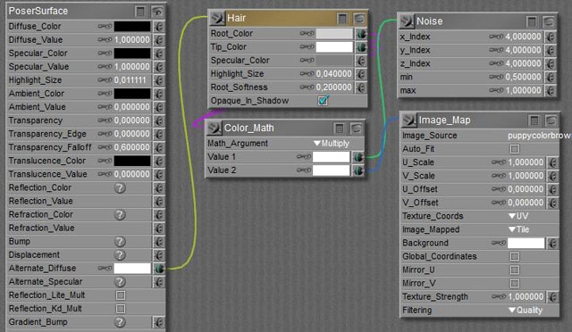
The cloth of the hat and muff are more complicated but essentially have the bluish grey tone as well, which is why the hair root material has quite a high Root Softness setting (0,5 instead of the default 0,1). The softness makes the hair roots transparent so they blend in well with the scull or surface, in this case with the cloth. If there is shadow on the cloth we might like the hair to stand out more, so the Opaque in Shadow is checked as well.

In Material Room is becomes clear that the 3D mesh (the cloth) of hat and muff are used to deliver the polys and vertices for the roots of the hairs, but the hairs themselves make a Prop to assign materials to.

Note that this prop cannot be saved, we are expected to save the hair growth surface with the (guide) hair definitions. This is what the hair collection in the Library expects.

CaseStudy: Hairy Stuff (5 Toon Animal)

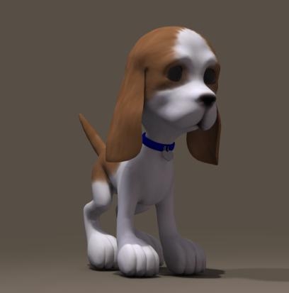
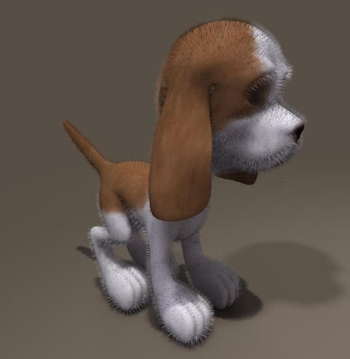
Next to clothing, animals are popular to assign fur too. To avoid debates on realism – which is mainly an issue of endless tuning of the grouping details, the hair parameters and the material properties – and since I’m a dog person, I’ll go for the Toon Puppy. For the cat persons amongst you, just take the Toon Kitten instead, or anything else.
The collar came as an additional prop, and I hide it for the moment.

There are two different ways to approach this:

Make a lot of small hair growth groups with different length and pull settings, and apply minor adjustments to them later
Make a few large growth groups without pull settings, and apply a lot of editing to the hairs themselves.

Making a choice upfront is relevant, because any attempt to alter a length or pull setting (Hair Room panel 2) erases all editing of hairs in that group. Since the Puppy is rather low poly and well curved, which implies: not that many guide hairs and a lot of detailed work required anyway, I take the second way. You might choose different for a highres Horse mesh.

Analysis

All areas that are worthwhile to be furrified are textured by mainly one (“Fur”) material, driven by a single image map. The Head consisted of a Fur, Muzzle and Nose material group, I picked the first two and left the latter out.

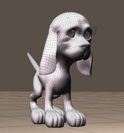
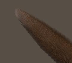
The puppy mesh offers the regular Head \ Neck \ Chest \ Abdomen \ Hip structure, and the four-part leg and arm structure. The fourth part is foot or hand, the puppy has no separate toes or fingers. The three-part ear-structure however is an addition to a normal (human) mesh, as is the ten-part tail. Especially this last element might do well with the straightforward Hair length and Pull settings, without additional editing.

Preparation
All this makes a 5+4*4+2*3+10=37 part animal, and each part gets its own hair growth group and hair material setting. Each hair growth group is a routine: select, [New Hair Group], [Edit Hair Group] using [Add All], [Grow Guide Hairs], set all values in panel 2 and 3, and [Grow Guide Hairs] again to make the preview properly show what I just did. Then next part.

The material is just a matter of setting up one correctly, and the copy / pasting as described in the Jacket chapter.

The skin image map is multiplied with the usual noise node, and fed into the Root color at a slightly darker tone than into the Tip color.

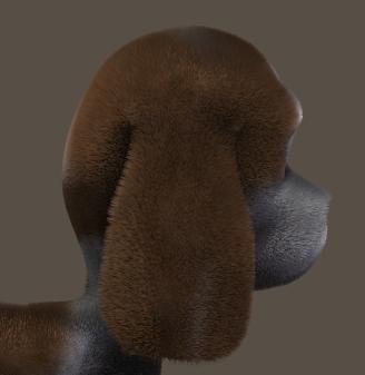
So after a tedious sequence of paste and [Remove Detached Nodes] in Material Room, I’ve got my Toon Puppy with guide hairs standing straight out on all places that should have hair. I excluded the bottom of feet and hand, excluded the nose on the head, and ensured that the inner parts of the ears were saved from hair by using the Fur material in my selections. And all hairs are colored properly. Time to save.

Styling
Now – except from hair density – our puppy or kitten only need his/her hair styled in the proper direction. As all surfaces are rather curved, the Pull values don’t serve that well and so I’ve to click [Style Guide Hairs] to use the Hair Editor. It’s just a matter of practice, and this animal offers almost 40 areas to practice with. The easiest parts are at the back (straight tail), the most varied and curved part is at the front (head). So, to gain experience along the way, I’ll work from the tail forward.

My main tools in the editor are the three ones up-left; select, deselect and move – which just pulls the hairs in a specific direction, plus the up-right one: scale – which tapers the hair ends. There is nothing to rotate, transfer or curl. I’ll keep all hairs at constant length while editing, all edits start at the hair roots (otherwise the hairs stand out for some part), and I won’t need to alter length, let alone exceptions at the ears or nose I guess. Each time I am dissatisfied (or just screw up), I can click [Grow Guide Hairs] in panel 2, and I can start all over again for that piece of hair.

Intermezzo
Since the puppy is composed from a lot of elements, it’s relevant that all have appropriate and matching parameters.

Length and variance are in user units. That is, if your general preferences (Interface tab) are set to inches, then 1.0 means; 1 inch. When you save your file, send it to me (I’ve my units set to meters), the same hair will show but the setting will read: 0,0254. Internally, Poser saves all lengths and distances in Poser Native Units (PNU). The translation is done in the user interface.
Pull is some angle between adjacent edges that make up a hair. The first edge always stand right up, then the bending starts. The more Verts per hair, the more edges, the more the hair will finally bend. And the smoother.
Hair density: the number next to the dial represents the amount of hairs per square user unit. If you (using inches) set it to 10 (hairs per square inch) and I open that file (using meters), I will see 16,000 in that field as 1 meter is about 40 inches (and 10x 40x 40 = 16,000). Note that human and animal hairs are about 100 hairs / cm2 = 645 hairs / inch2 = 1,000,000 hairs/m2. The number between brackets tells the amount of hairs to be generated in the population.
The hair objects generated by Hair Room might become really huge for realistic settings at a high Verts per hair count. A Gorilla, having a body surface of say 2 m2, at 1 million hairs per m2, and 8 verts per hair will generate 16 million vertices which is 200 times as much as a highres Vicky character. You and your PC need the resources (memory, CPU power, render time) to handle that.
Note that the default reads 32,000 hairs per square PNU = 4300 per m2 = 3 per square inch, that’s way below the natural values.
Anyway, when all elements of the puppy needs matching settings, so needs Hair Density to be similar for all of them.
Width, at the tip and the root, can be considered in mm. For natural hair, 0.1 is a decent (root) value.
(thought experiment: take 1 cm2 of surface, give it 100 hairs in a matrix at equal distance, and look straight at it (Front camera or alike). Then 10% of the area looks filled up, as 100 = 10×10, and 10 hairs of 0.1 mm make 1mm = 10% of 1 cm. So a setting of 1 (mm) is really thick.
But when you choose – for performance reasons – for a lower Density setting you can take higher width values to compensate, until things start looking unnatural.
Kink makes curls in a hair, the Scale sets the number of them over a full length, so 4.0 makes 3 full waves as 1.0 makes no wave at all. A delay of 0.2 makes the first 20% from the root up without curl, only the 80% to the tip are effected. More curls per hair require a sufficient setting for the Verts per hair, 4 verts per kink is a minimum to experience effects of some quality (so scale =4 makes about 16 verts minimum), below that the hair gets fuzzy. Strength makes just stronger curls.
Verts per hair was discussed already, the more you use the more PC power you need to render the result, the smoother and more natural it looks (always that same trade-off J ), the more effect you’ll get from the same Pull values, and the better the quality from Kinks.

Getting Results
Back to Toon Puppy. When I set all hair groups to 1,000,000 hairs per m2, and counted all hairs generated from that, I found that my Toon Puppy was going to end up with about 1,370,000 hairs @16 verts/hair = 22,000,000 vertices. Pressing Render revealed that the memory requirements for even a shadow map went towards 20Gb RAM user memory, causing my PC to start disk-swapping. Not good. Reducing the density a tenfold to 100,000 / m2 reduced the RAM requirements to say 2Gb, easy on my machine but in my opinion a bit too low on quality at close-up camera distance.

So you can make a compromise depending on your machine specs. See the images, 500,000 hairs/m2, head unstyled, tail styled). Watch the (Windows) TaskManager to flag issues and chances.
By the way: after the tenfold reduction, Toon Puppy had as many hairs as a human blonde (150,000) so Poser is well equipped to handle nice portraits etc at a quality representing nature.

And of course, I can bring down the Verts/hair from 16 to 12 (or 8?). but that is something I can do best before creating styles with the Hair Editor. So, mind the numbers (or just watch TaskManagers when things tend to go wrong), and make some test renders to find the quality balance. High end (large size, high quality) results require appropriate machines, sorry for that.

Styling tip: in many cases, there is no One Style that fits all hairs in the group. Like this tail part, the hairs towards the tip end are a bit more styled than the hairs towards the body end, which are more upright. I handle this by first selecting all, do some styling, deselect hairs at the body side, style a bit, deselect more, style a bit, and so on. Especially the Hip (meeting tail and both legs) and the head (lots of curves) need threatments like that.

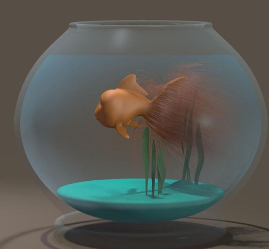
Toon Fish
I know, most fish don’t have hair, but a hairy toon fish helps me to introduce some dynamics (panel 4).

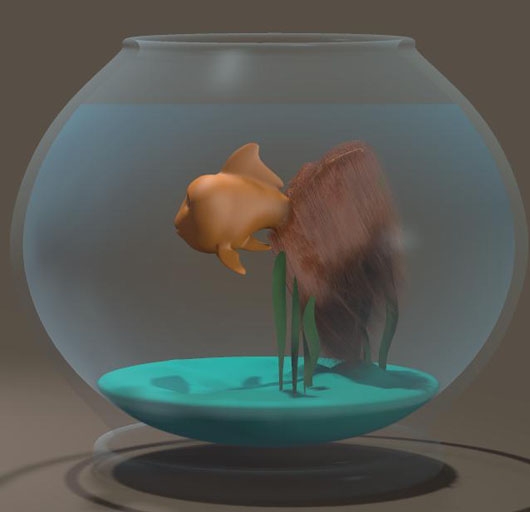
I simply select the tail, assign it a Hair Group, grow guide hairs and turn them orange for the fit. At 40cm length, some Pull back and down, with some density (20,000/m2), and no Kinks, this is it:

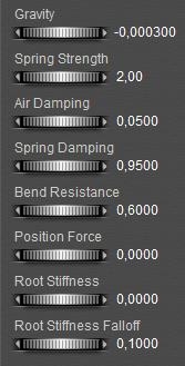
In panel 4, I reduce the Bend Resistance, zero the Root Stiffness and reduce the Falloff.
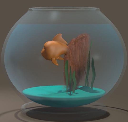
I click [Calculate Dynamics], gravity takes the hairs down, but the default 30 frames are not enough.

So I double them, to 60:

And I [Calculate Dynamics] again.

Nice, but a bit boring:

So I added a ForceField (menu Object . Add Wind Force). I put it about in front of the fish, and adjusted its parameters:

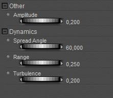
And I unchecked Visible in Camera, as the ForceField should look as being generated by the swimming.

And I [Calculate Dynamics] again. Better, but let’s give it another try: Turbulence up to maximum (1.0), and after the calculation I use the time slider to seek an interesting frame. Halfway, I’ve got one for render. To spice it up even more, you can try the workings of the Wave generator (menu Objects . Add Wave). Next time you make dynamic hair for your swimming mermaid, think about the hairy goldfish. Golden hairfish. Whatever.